


Development, study, and comparison of models of cross-immunity to the influenza virus using statistical methods and machine learning
- Authors: Asatryan M.N.1, Shmyr I.S.1, Timofeev B.I.1, Shcherbinin D.N.1, Agasaryan V.G.1, Timofeeva T.A.1, Ershov I.F.1, Gerasimuk E.R.1,2, Nozdracheva A.V.1, Semenenko T.A.1, Logunov D.Y.1, Gintsburg A.L.1
-
Affiliations:
- National Research Center for Epidemiology and Microbiology named after Honorary Academician N.F. Gamaleya
- State University «Dubna»
- Issue: Vol 69, No 4 (2024)
- Pages: 349-362
- Section: ORIGINAL RESEARCHES
- URL: https://virusjour.crie.ru/jour/article/view/16667
- DOI: https://doi.org/10.36233/0507-4088-250
- EDN: https://elibrary.ru/phejeu
- ID: 16667

Cite item

Abstract
Introduction. The World Health Organization considers the values of antibody titers in the hemagglutination inhibition assay as one of the most important criteria for assessing successful vaccination. Mathematical modeling of cross-immunity allows for identification on a real-time basis of new antigenic variants, which is of paramount importance for human health.
Materials and methods. This study uses statistical methods and machine learning techniques from simple to complex: logistic regression model, random forest method, and gradient boosting. The calculations used the AAindex matrices in parallel to the Hamming distance. The calculations were carried out with different types and values of antigenic escape thresholds, on four data sets. The results were compared using common binary classification metrics.
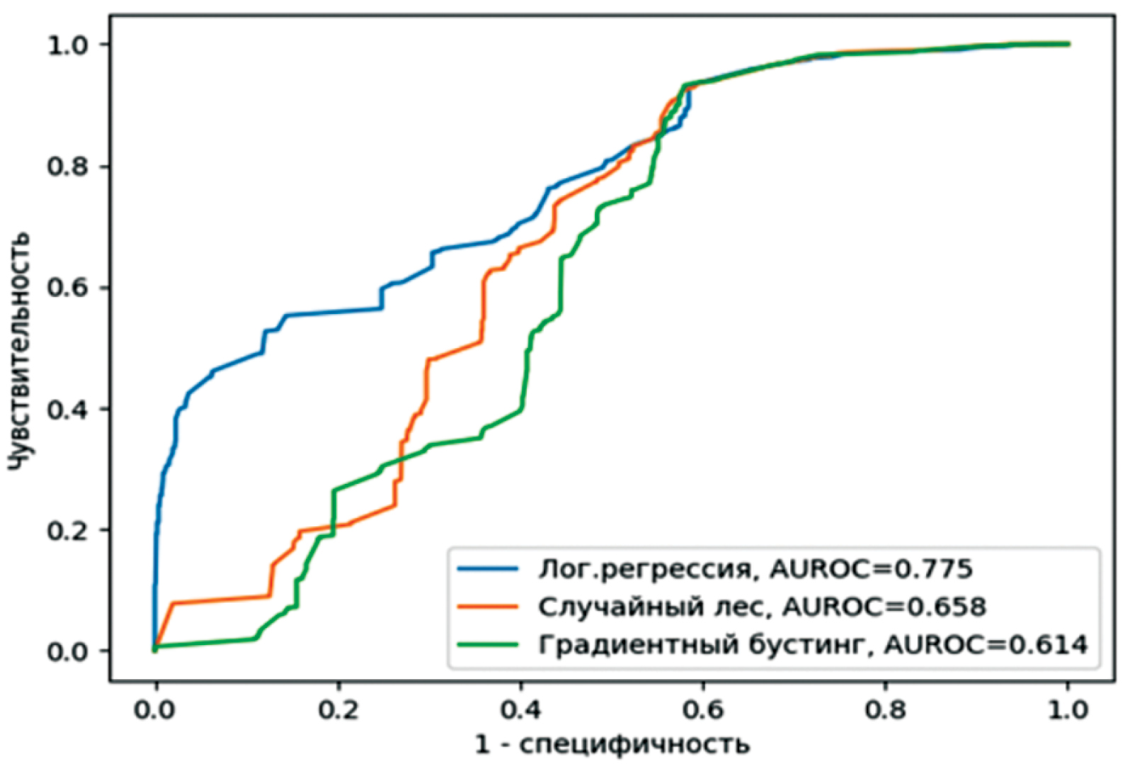
Results. Significant differentiation is shown depending on the data sets used. The best results were demonstrated by all three models for the forecast autumn season of 2022, which were preliminary trained on the February season of the same year (Auroc 0.934; 0.958; 0.956, respectively). The lowest results were obtained for the entire forecast year 2023, they were set up on data from two seasons of 2022 (Aucroc 0.614; 0.658; 0.775). The dependence of the results on the types of thresholds used and their values turned out to be insignificant. The additional use of AAindex matrices did not significantly improve the results of the models without introducing significant deterioration.
Conclusion. More complex models show better results. When developing cross-immunity models, testing on a variety of data sets is important to make strong claims about their prognostic robustness.
Full Text
Introduction
It is well known that the influenza A virus, belonging to the Orthomyxoviridae family [1], has high mutational variability; therefore, circulating strains (populations) include mutant variants that avoid the protective effect of antibodies developed both as a result of the disease and vaccination. Mutant forms of the virus that carry certain substitutions and lead to conformational changes in the surface protein can cause difficulties in the interaction of antigenic sites with neutralizing antibodies, which is important when selecting and evaluating strains for creating vaccines.
The World Health Organization (WHO) considers the values of antibody titers in the hemagglutination inhibition assay (HIA) as one of the most important criteria for assessing successful vaccination and the ability to prevent disease in the population1. At the same time, laboratory experimental studies are quite time-consuming and labor-intensive. Mathematical modeling of cross-immunity allows for identification on a real-time basis of new antigenic variants, which is of paramount importance for epidemiological surveillance and human health [2, 3].
A promising direction is modelling the spread of the influenza virus over long time intervals, taking into account seasonality and mutation factors, to recommend a vaccine strain for the upcoming season. In 2020, the team of the National Research Center for Epidemiology and Microbiology named after N.F. Gamaleya developed and successfully registered the Influenza IDE software (a multi-strain epidemic model (MEM)) with a cross-immunity model and a constantly updated database Influenza DB of various types and subtypes of the virus [4]. The MEM uses a population (agent) model to simulate the spread of the influenza virus among the population, as well as nested models (cross-immunity and immune response) to form an immune landscape (is the quantitative distribution of antigenic variants (with antibodies produced against them) among the population at a given point in time in accordance with the individual disease histories of agents (individuals)), that directly affects the speed and extent of spread of individual influenza virus strains among the population and recommend the most effective vaccine strain. The software is designed to be able to integrate multiple models of cross-immunity [5]. As part of research on modifying the software, the team of authors is developing models of cross-immunity, using the example of the influenza A (H3N2) virus, incorporating mathematical methods.
The purpose of the study is to develop, study, and compare cross-immunity models using statistical methods and machine learning.
Materials and methods
Data description
To develop models and calculations, the Influenza DB data set was used with information from:
‒ Published WHO seasonal data on the results of serum testing in the HIA (the entire data set from 2014‒2023 of both reference and test strains of influenza A (H3N2) virus);
‒ From the GISAID (Global Initiative on Sharing All Influenza Data) platform (sequences + supporting information).
After cleaning and harmonizing the data from GISAID, followed by alignment to the reference sequence and combining into antigenic sites, according to the proposed proprietary template, a Hamming distance matrix was formed for each of the 6 antigenic sites (with assignment of a unique identifier to each sequence).
In previous calculations [5], by tuning and forecast based on later data, we showed that the accuracy of the results is significantly influenced by the volume and quality of the HIA studies performed. To develop models of cross-immunity, the subset with the largest number (36,509) of Cell-Cell observations (with passage history in cell culture) was selected. Taking into account the fundamental increase in observations in 2022 and 2023, we decided to choose the said seasons as forecast periods. While the intervals from 2014‒2021, as well as 2022 and 2023, respectively, were taken as retrospective tuned periods (Table 1).
Table 1. Data characteristics
Таблица 1. Характеристика данных
Model training / Обучение модели | Model testing / Тестирование модели | ||||
period период | number of strain pairs число пар штаммов | titer титр | period период | number of strain pairs число пар штаммов | titer титр |
2014‒2021 | 10 272 | 160 [40; 320] | 2022 | 8183 | 80 [40; 320] |
2022 | 8183 | 80 [40; 320] | 2023 | 6143 | 160 [80; 320] |
2023 (feb.) / (фев.) | 2518 | 80 [40; 320] | 2023 (sep.) / (сен.) | 3689 | 160 [80; 320] |
2022 (feb.) / (фев.) | 1994 | 160 [40; 320] | 2022 (sep.) / (сен.) | 6675 | 80 [40; 320] |
In previous calculations, integer numeric values were used as Hamming distance values according to the number of amino acid substitutions (for example, 0, 1, 2, 3 … 8). For a more sensitive assay, assessment of the contribution of each amino acid and comparison, we used the AAindex matrices in this study. This is a database of numerical indicators reflecting various physical-chemical and biochemical properties of amino acids and amino acid pairs. Thus, in parallel, replacing the value of the Hamming distance with the inherent numerical value of a specific physical-chemical characteristic.
The AAindex database consists of three sections and is released every year. The matrices are presented as flat files: AAindex1 for amino acid indices, AAindex2 for amino acid substitution matrices, and AAindex3 for amino acid contact potentials. Currently, researchers continue to collect and complete the database, following the expansion of the collection2 [6].
Determination of antigenic distance and selection of thresholds
The common «gold standard» for assessing the presence and determining the concentration of virus-neutralizing antibodies in studied serum specimens is the hemagglutination inhibition assay (HIA). Essentially, the HIA assesses the level of cross-immunity against the influenza virus [7‒9].
A significant number of studies on the investigation of antigenic differences between strains (antigenic distance) use both the titer values themselves and various expressions from the HIA titers or logarithms from these expressions: Rij = cij / cii [10]; log2(Rij), as a measure of cross-immunity during infection and/or to study the effectiveness of vaccines [11‒13]. In the meantime, certain values of these titers and expressions may indicate the presence or absence of protection against infection with a specific strain of influenza virus. And, in this case, the transition value is called the antigenic escape threshold. For the current study, we determined the values of the probabilistic thresholds of antigenic escape, expressed in titers, referring to scientific literature data, as 1 : 40 and 1 : 80. [14, 15].
In addition, it is well known that the results are significantly influenced by the individual characteristics of laboratory animals. To reduce the influence of these factors, it is not the titer value itself that is taken as the threshold for antigenic escape, but the ratio of the titer in the reaction under consideration, normalized to its maximum dilution for a given serum. In this study, we decided to carry out calculations for the entire array of test strains and take the ratio of the maximum titer value in the experiment to the titer value of the test strain as the thresholds for antigenic escape (ref_max/titer) greater than 4; and greater than or equal to 4 [12, 13, 16–19].
Thus, for further calculations, antigenic escape thresholds were used, expressed in titers (dilutions 1:40; 1:80) and normalized (ref_max/titer > 4; ref_max/titer ≥ 4).
Cross-immunity models
For the chosen purpose and to solve binary classification problems (in our case, antigenic escape), statistical methods and machine learning techniques were considered: from simple to complex, such as the logistic regression model, the random forest method and the gradient boosting.
Logistic regression is a type of statistical modelling that allows one or more independent variables (predictors) to be quantitatively associated with a binary attribute by determining the odds ratio of possible outcomes [20].
Random forest method is a machine learning algorithm that uses an ensemble of decision trees. Decision trees are a nonparametric algorithm used to solve classification and regression problems. The algorithm works based on the principle of a tree structure, where each internal node represents a test for the value of some attribute, each branch is the result of this test, and each leaf node is a class mark or numeric value. The random trees method assigns the object to the class that was selected by the majority of decision trees included in the ensemble3.
Gradient boosting is a machine learning technique that is used for classification and regression problems. The main idea of gradient boosting is to construct an ensemble of weak models, usually decision trees, in such a way that each subsequent model corrects the errors of the previous models [21]. As part of this study, the CatBoost library was used to implement gradient boosting4 .
Python programming language libraries were used for data preprocessing, descriptive statistics, learning and quality assessment of the models:
‒ pandasql 0.7.3 – data preprocessing;
‒ pandas 2.0.3 – descriptive statistics, presentation of results;
‒ sklearn 1.2.2 – logistic regression, random forest method, model quality assessment
‒ matplotlib 3.7.1 – plots.
The analysis of the stability of the predictive ability of cross-immunity models was carried out on retrospective data with the largest number of observations with subsequent forecast. As a measure of the adequacy (quality and accuracy of forecast) of models and comparison of various algorithms, quality metrics adopted in machine learning tasks were used (indicators that depend on the classification results and do not depend on the internal state of the model):
‒ Accuracy is the percentage of reproducibility of correct model results;
‒ Sensitivity (completeness) or True Positive Rate (TPR) is defined as the number of true positive classifications relative to the total number of positive observations;
‒ Specificity is the proportion of True Negatives Rate (TNR) defined as the number of true negative classifications in the total number of negative classifications;
‒ MCC (Matthews Correlation Coefficient) is a balanced measure of performance that can be used even if a class includes many more samples than another one. Value range from −1 to +1;
‒ F1 (F-score) is a balanced metric that combines information about accuracy (precision) and sensitivity (completeness) using their harmonic mean value. Maximization of F1 is achieved when completeness and accuracy are simultaneously equal to 15,6.
The ROC analysis was also used as the most comprehensive indicator of model adequacy. The ROC curve shows the dependence of the number of correctly classified positive examples on the number of incorrectly classified negative examples. A quantitative interpretation of the ROC analysis is provided by the AUC indicator (Area Under Curve, area under the ROC curve). The higher the AUROC score, the better the classifier. The following gradation is normally used: Excellent (0.9‒1.0); Very good (0.8‒0.9); Good (0.7‒0.8); Average (0.6‒0.7); Unsatisfactory (0.5‒0.6)7,8.
The studies were carried out according to the design presented in Figure 1.

Fig. 1. Study flowchart. 1.1. Selection of source data; 1.2. Selecting the threshold for antigen release; 1.3. Dividing the data into a training and a forecast periods; 2. Model development; 3. Adequacy assessment and comparative analysis. Explanations in the text.
Рис. 1. Блок-схема исследования. 1.1. Выбор исходных данных; 1.2. Выбор порога антигенного ускользания; 1.3. Разделение данных на обучающий период и прогнозный; 2. Построение моделей; 3. Оценка адекватности и сравнительный анализ. Пояснения в тексте.
Results
In our study, the binary classification implemented by various methods (logistic regression model, random forest and gradient boosting) is used to predict the probability of occurrence of a certain outcome (protected or not) based on titer values in dilutions (1 : 40; 1 : 80) or normalized ones (ref_max/titer > 4; ref_max/titer ≥ 4).
Thresholds expressed in titers (dilutions 1 : 40 and 1 : 80)
As the threshold value of cross-immunity between two arbitrary strains in our calculations, we decided to take the value of the HIA titer in dilutions of both 40 and 80.
The distribution of the positive attribute (antigenic escape) for the 1 : 40 and 1 : 80 thresholds in both all tuned and forecast periods ranged from 30 to 40% and from 47 to 53%, respectively. The exception was year 2023, where the ranking of the same attribute varied from 37 to 44% for the 1 : 80 threshold, and from 15 to 26% for the 1 : 40 threshold. Detailed information for all thresholds and periods is presented in the Appendix.
For each time period, all three models were tuned and tested according to the study design. The calculation results for all three models in titers (1 : 40) are presented in Table 2 and in Plots (Fig. 2‒5). The adequacy of each model for the selected forecast periods was assessed using common indicators.
Table 2. Threshold titer (1 : 40)
Таблица 2. Порог в титрах (1 : 40)
Parameter Параметр | Accuracy | Sensitivity | Specificity | MCC | F1 | AUROC |
2014‒2021 => 2022 | ||||||
Logistic regression Лог. регрессия | 0.764 | 0.704 | 0.858 | 0.548 | 0.785 | 0.859 |
Random forest Случайный лес | 0.803 | 0.727 | 0.924 | 0.635 | 0.819 | 0.886 |
Gradient boosting Градиентный бустинг | 0.814 | 0.750 | 0.913 | 0.647 | 0.831 | 0.899 |
2022 (фев. / feb.) => 2022 (sep. / сен.) | ||||||
Logistic regression Лог. регрессия | 0.861 | 0.804 | 0.949 | 0.735 | 0.875 | 0.934 |
Random forest Случайный лес | 0.886 | 0.931 | 0.815 | 0.759 | 0.909 | 0.958 |
Gradient boosting Градиентный бустинг | 0.880 | 0.944 | 0.781 | 0.747 | 0.906 | 0.956 |
2023 (feb. / фев.) => 2023 (sep. / сен. ) | ||||||
Logistic regression Лог. регрессия | 0.637 | 0.607 | 0.806 | 0.297 | 0.739 | 0.760 |
Random forest Случайный лес | 0.734 | 0.719 | 0.815 | 0.399 | 0.821 | 0.854 |
Gradient boosting Градиентный бустинг | 0.869 | 0.953 | 0.402 | 0.420 | 0.925 | 0.851 |
2022 => 2023 | ||||||
Logistic regression Лог. регрессия | 0.837 | 0.970 | 0.304 | 0.393 | 0.905 | 0.775 |
Random forest Случайный лес | 0.838 | 0.968 | 0.316 | 0.398 | 0.905 | 0.658 |
Gradient boosting Градиентный бустинг | 0.837 | 0.968 | 0.311 | 0.395 | 0.905 | 0.614 |

Fig. 2. 2014‒2021 => 2022 (1 : 40). Here and in Fig. 3–5: the logistic regression model is shown in blue; random forest – in yellow; gradient boosting – in green, for one type of threshold expressed in titers (dilution 1 : 40). The sensitivity is plotted on the Y-axis, and the 1 minus specificity represent on the X-axis. Explanations are given in the text.
Рис. 2. 2014‒2021 => 2022 (1 : 40). Здесь и на рис. 3‒5: модель логистической регрессии выделена синим цветом; случайного леса ‒ желтым цветом; градиентного бустинга ‒ зеленым цветом, для одного типа порога, выраженного в титрах (разведение 1 : 40). По оси У отложена чувствительность (sensitivity), а по оси Х отложена: 1 минус специфичность (specificity). Пояснения в тексте.

Fig. 3. 2022 (feb.) => 2022 (sep.) (1 : 40).
Рис. 3. 2022 (фев.) => 2022 (сен.) (1 : 40).

Fig. 4. 2023 (feb.) => 2023 (sep.) (1 : 40).
Рис. 4. 2023 (фев.) => 2023 (сен.) (1 : 40).

Fig. 5. 2022 => 2023 (1 : 40).
Рис. 5. 2022 => 2023 (1 : 40).
As can be seen from the results, more complex models show better results in almost all indicators. The results for the forecast period of 2023, with a pre-set period for 2022, stand out from this series with a slight difference. Regarding the comparison of individual indicators across all three models, attention should be paid to the (values of) specificity and sensitivity. Both metrics are balanced for all forecast and tuned periods. The exception is the forecast period of year 2023, tuned on year 2022, which exhibits high values for sensitivity and low values for specificity.
Figures 2‒5 show the results of the ROC analysis of all three models. According to the adopted metric of classifier quality, the good performance under the ROC curve is illustrated by all three models for the forecast year 2023 with preliminary learning on data for year 2022. Very good results were obtained for the tuned period from 2014 to 2021 with a forecast for 2022. The forecasted September 2023 season, which was pre-tuned for the February period of the same year, showed similar results. The results of all three models for the forecast autumn season of year 2022 are quite stable. Models trained on the February season of year 2022 demonstrated excellent AUROC values. These results coincide with our own indicators based on multiple linear regression [5].
We also decided to test the quality of our models for a cross-immunity titer threshold value equal to 80. Detailed calculations (tables, ROC curves) are presented in the Appendix.
When comparing the results obtained using different threshold escape values, attention is drawn to the fact that, regardless of the threshold value, the same trends remain for all tuned periods: the best results were obtained in the forecast for 2022 and slightly moderate ones in the forecast for 2023.
Thresholds expressed by the ratios ref_max/titer > 4 and ref_max/titer ≥ 4)
As has been noted more than once by researchers, despite all efforts to standardize the HIA [22], the initially high error of the HIA technique (17%) [23] remains a factor that significantly influences the results. In addition, the final result is significantly influenced by the individual characteristics of laboratory animals. To reduce the influence of these factors, we used the normalized ratio ref_max/titre > 4 and ≥ 4 as the threshold for antigenic escape in our calculations.
There is a fairly even distribution of the positive attribute (antigenic escape) for the normalized threshold ref_max/titre > 4 in both all tuned and forecast periods from 44 to 54%. For the normalized threshold ref_max/titre ≥ 4, the ranking of the same attribute changes from 21 to 28%. Detailed information is provided in the Appendix.
As can be seen from Table 3, the trends continue with the results of calculations using the threshold equal to 40. As in the previous case, the results for the forecast period of year 2023, with a pre-set period of year 2022, differ from the general trend.
Table 3. Threshold normalized more than 4
Таблица 3. Нормированный порог больше 4
Parameter Параметр | Accuracy | Sensitivity | Specificity | MCC | F1 | AUROC |
2014‒2021 => 2022 | ||||||
Logistic regression Лог. регрессия | 0.817 | 0.915 | 0.714 | 0.644 | 0.836 | 0.840 |
Random forest Случайный лес | 0.816 | 0.893 | 0.736 | 0.638 | 0.832 | 0.861 |
Gradient boosting Градиентный бустинг | 0.821 | 0.900 | 0.738 | 0.648 | 0.837 | 0.899 |
2022 (feb. / фев.) => 2022 (sep. / сен.) | ||||||
Logistic regression Лог. регрессия | 0.883 | 0.929 | 0.837 | 0.769 | 0.888 | 0.942 |
Random forest Случайный лес | 0.890 | 0.897 | 0.883 | 0.780 | 0.891 | 0.951 |
Gradient boosting Градиентный бустинг | 0.890 | 0.904 | 0.876 | 0.781 | 0.892 | 0.951 |
2023 (feb. / фев.) => 2023 (sep. / сен.) | ||||||
Logistic regression Лог. регрессия | 0.750 | 0.791 | 0.715 | 0.505 | 0.745 | 0.821 |
Random forest Случайный лес | 0.770 | 0.840 | 0.710 | 0.550 | 0.771 | 0.849 |
Gradient boosting Градиентный бустинг | 0.762 | 0.804 | 0.726 | 0.528 | 0.757 | 0.848 |
2022 => 2023 | ||||||
Logistic regression Лог. регрессия | 0.624 | 0.249 | 0.965 | 0.310 | 0.386 | 0.664 |
Random forest Случайный лес | 0.613 | 0.257 | 0.938 | 0.268 | 0.388 | 0.748 |
Gradient boosting Градиентный бустинг | 0.614 | 0.259 | 0.937 | 0.268 | 0.389 | 0.725 |
Figures 6‒9 present the results of the ROC analysis of all three models for the normalized threshold (> 4).

Fig. 6. 2014‒2021 => 2022 (> 4). Here and in Fig. 7–9: logistic regression models are shown in blue; random forest models are shown in yellow; gradient boosting models are shown in green. Sensitivity is plotted on the Y-axis, and 1 minus specificity represents on the X-axis. Explanations are given in the text.
Рис. 6. 2014‒2021 => 2022 (> 4). Здесь и на рис. 7‒9: модели логистической регрессии выделены синим цветом; случайного леса ‒ желтым цветом; градиентного бустинга ‒ зеленым цветом. По оси У отложена чувствительность (sensitivity), а по оси Х отложена: 1 минус специфичность (specificity). Пояснения в тексте.

Fig. 7. 2022 (feb.) => 2022 (sep.) (> 4).
Рис. 7. 2022 (фев.) => 2022 (сен.) (> 4).

Fig. 8. 2023 (feb) => 2023 (sep.) (> 4).
Рис. 8. 2023 (фев) => 2023 (сен.) (> 4).

Fig. 9. 2022 => 2023 (> 4).
Рис. 9. 2022 => 2023 (> 4).
At all forecast periods, the values of the areas under the ROC curves are above 0.8, as in the case of calculations for thresholds expressed in titers (1 : 40 and 1 : 80), with the exception of the plots in Figure 9, where the AUROC value is above 0.7 for random forest and gradient boosting models.
The main reason for the lower AUROC score is the low sensitivity of the models. It should be noted that, in contrast to the threshold type (1 : 40 and 1 : 80) for the period tuned on the data of year 2022 and the forecast for year 2023, logistic regression shows a lower result than in the case of more complex models
The results for the normalized threshold greater than and equal to 4 are generally similar for all periods, but, as expected, have higher sensitivity and weaker specificity. The difference is especially noticeable in the forecast for year 2023 tuned on data of year 2022. Full calculations are presented in the Appendix.
Application of AAindex matrices
At the next stage of research, we applied the AAindex matrices, thereby replacing the value of the Hamming distance with the inherent numerical value of a specific physical-chemical and biochemical characteristic. Foreign colleagues used AAindex matrices in various combinations in their studies. They are presented in quite a significant number. And we considered it useless to apply all the matrices without a validated theory or logic. Therefore, as a starting point, it was decided to use the most frequently intersecting matrices that showed the best results with the colleagues [24‒27] and then compare the results obtained:
‒ AZAE970101 The single residue substitution matrix from interchanges of spatially neighbouring residues (Azarya-Sprinzak et al., 1997).
‒ BENS940104 Genetic code matrix (Benner et al., 1994).
‒ MUET010101 Non-symmetric substitution matrix (SLIM) for detection of homologous transmembrane proteins (Mueller et al., 2001).
The calculation results for all three models, for the threshold in titers (1 : 40) and normalized greater than 4, are presented in Tables 4 and 5. All the other calculations are presented in the Appendix.
Table 4. Threshold titer (1 : 40). Сomparison of results
Таблица 4. Порог в титрах (1 : 40). Сравнение результатов
Parameter Параметр | Hamming distance Дистанция Хемминга | AAindex-AZAE_40 | AAindex-BENS_40 | AAindex-MUET_40 |
AUROC | AUROC | AUROC | AUROC | |
2014‒2021 => 2022 | ||||
Logistic regression Лог. регрессия | 0.850 | 0.856 | 0.857 | 0.874 |
Random forest Случайный лес | 0.879 | 0.876 | 0.878 | 0.878 |
Gradient boosting Градиентный бустинг | 0.893 | 0.894 | 0.908 | 0.898 |
2022 (feb. / фев.) => 2022 (sep. / сен.) | ||||
Logistic regression Лог. регрессия | 0.912 | 0.887 | 0.937 | 0.932 |
Random forest Случайный лес | 0.958 | 0.956 | 0.958 | 0.957 |
Gradient boosting Градиентный бустинг | 0.956 | 0.957 | 0.959 | 0.957 |
2023 (feb. / фев.) => 2023 (sep. / сен.) | ||||
Logistic regression Лог. регрессия | 0.772 | 0.796 | 0.758 | 0.790 |
Random forest Случайный лес | 0.854 | 0.882 | 0.886 | 0.884 |
Gradient boosting Градиентный бустинг | 0.851 | 0.883 | 0.878 | 0.875 |
2022 => 2023 | ||||
Logistic regression Лог. регрессия | 0.790 | 0.685 | 0.749 | 0.737 |
Random forest Случайный лес | 0.659 | 0.654 | 0.659 | 0.649 |
Gradient boosting Градиентный бустинг | 0.624 | 0.629 | 0.581 | 0.590 |
Table 5. Threshold normalized more than 4. Сomparison of results
Таблица 5. Нормированный порог больше 4. Сравнение результатов
Parameter Параметр | Hamming distance Дистанция Хемминга | AAindex-AZAE ref_max/titre >4 | AAindex-BENS ref_max/titre >4 | AAindex-MUET ref_max/titre >4 |
AUROC | AUROC | AUROC | AUROC | |
2014‒2021 => 2022 | ||||
Logistic regression Лог. регрессия | 0.821 | 0.833 | 0.762 | 0.821 |
Random forest Случайный лес | 0.876 | 0.881 | 0.880 | 0.884 |
Gradient boosting Градиентный бустинг | 0.899 | 0.884 | 0.904 | 0.908 |
2022 (feb. / фев.) => 2022 (sep. / сен.) | ||||
Logistic regression Лог. регрессия | 0.936 | 0.902 | 0.944 | 0.943 |
Random forest Случайный лес | 0.950 | 0.941 | 0.948 | 0.947 |
Gradient boosting Градиентный бустинг | 0.951 | 0.946 | 0.950 | 0.943 |
2023 (feb. / фев.) => 2023 (sep. / сен.) | ||||
Logistic regression Лог. регрессия | 0.819 | 0.821 | 0.820 | 0.823 |
Random forest Случайный лес | 0.848 | 0.842 | 0.846 | 0.841 |
Gradient boosting Градиентный бустинг | 0.848 | 0.844 | 0.849 | 0.848 |
2022 => 2023 | ||||
Logistic regression Лог. регрессия | 0.740 | 0.575 | 0.644 | 0.709 |
Random forest Случайный лес | 0.734 | 0.732 | 0.739 | 0.747 |
Gradient boosting Градиентный бустинг | 0.714 | 0.714 | 0.676 | 0.736 |
Based on the comparative results presented in Tables 4, 5, it can be stated that the AUROC scores calculated both using the Hamming distance and the selected AAindex matrices do not differ significantly. Noteworthy is the fact that the generally followed rule is: more complex models demonstrate better results, including the forecast for the period of year 2023, tuned on data from year 2022, with the normalized threshold greater than > 4. This rule works better for calculations with the AAindex matrices, with only a few exceptions. Results of the full study are presented in the Appendix.
Discussion
The main purpose of this study was to investigate the influence on the study results of different types of cross-immunity models used. For a more objective and stable assessment, we trained and tested the models that we had developed over various time periods. In this case, both the type of antigenic escape threshold and its value were varied.
Generally, as expected, more complex models showed better results. The only time period using the threshold type expressed in titers (1 : 40; 1 : 80), which stands out from this pattern, is the results for the forecast period of year 2023 with a pre-tuned period of year 2022, where the best result was shown by the simplest logistic regression model. At the same time, it is important to note that our calculations clearly demonstrated the significant influence of the time periods under consideration, i.e. data arrays, on forecast results.
The best forecast results, using all types of models and different types of antigenic escape threshold values, were obtained for the September season of year 2022, pre-tuned on the February season. Good forecast results for the full year 2022 were demonstrated by the models trained on data from 2014 to 2021. Next, in descending gradation, the results of the forecast for the February period of year 2023 are presented, with the tuned September season of the same year. And the lowest values were shown by calculations for the full year 2023, with training on data from two seasons of 2022.
Comparing results using different types of antigenic escape thresholds does not reveal significant differences. At the same time, in should be noted that for the threshold values, in titers (1 : 80) and normalized > 4, the distribution of the studied attribute of antigenic escape (positive outcome) is more uniform, from 37 to 54%, respectively. A slightly different, sharper distribution of the positive outcome (from 15 to 40%) is demonstrated by the results obtained for threshold values in titers (1 : 40) and normalized ≥ 4.
Also attracting attention is the fact that when replacing the threshold value, expressed both in titers and normalized, from a smaller value to a larger one, two specific parameters for assessing models – sensitivity and specificity – are somewhat interrelated. In calculations, the sensitivity increases and the specificity decreases.
For the first time, very high forecast results for the September season of year 2022, with a pre-tuned model on February data of the same year, were obtained in our study [5], using an unprecedented amount of data for year 2022. In the present study, we repeated the calculations in a similar way, but using the developed new models. Additionally, similar calculations were carried out with data for year 2023. In both cases, good results were obtained. The robustness of the proposed approach needs to be tested using data from subsequent seasons.
The active use of the AAindex databases in the development of cross-immunity models has been noted in a number of scientific papers in recent years [24‒27]. Since the AAindex matrices include numerical indicators reflecting various physical-chemical properties of amino acids and amino acid pairs, we can presume that their use in calculations should lead to improved model accuracy.
Our calculations using three AAindex matrices selected on the basis of the most frequently intersecting matrices in several foreign scientific papers, did not show a significant improvement in the results. It should be noted that using them did not worsen the results.
The above may indicate that the objective assessment of the results in case of using specific AAindex matrices requires a biological justification of the rationale for applicability of them in a particular case.
In the studies on cross-immunity model development published to date, researchers typically use one set of data to train the model on and test it on another set of data. In some cases, the entire sample (set of data) is randomly divided into two parts, with a larger volume intended for tuning the model and a smaller quantity for validation [13, 16, 24, 27‒31]. The results of the current study show that such an algorithm is not sufficient to justify the predictive ability of the model. Our calculations suggest that the results differ quite significantly depending on the data sets used. In our opinion, to overcome this limitation and make a convincing statement about the prognostic robustness of the model, it is necessary to carry out both tuning and testing on several different sets.
Conclusion
In current research, more complex models developed by statistical methods and machine learning have demonstrated better results. At the same time, selective application of types of antigenic escape thresholds and replacement of their numerical values do not make a significant contribution. They should be selected based on factors independent of the model itself.
It is important and necessary to train and test cross-immunity models based on searching for the dependence of HIA titers on changes in amino acid positions of influenza virus sequences on various data sets.
The existing knowledge base and skills of researchers in both technical and biological areas allow for further development of models of cross-immunity, using more complex deep learning techniques.
Funding. This study was not supported by any external sources of funding.
Acknowledgements. We gratefully acknowledge the staff of the N.F. Gamaleya Center, Chief Researcher F.I. Ershov, Head of the Department of Virus Ecology at the Ivanovskiy Institute of Virology E.I. Burtseva, Head of the Laboratory of Molecular Biotechnology M.M. Shmarov, Leading Researcher at the Laboratory of Virus Physiology of the Ivanovskiy Institute of Virology I.A. Rudneva for numerous consultations during the study.
Conflict of interest. The authors declare no apparent or potential conflicts of interest related to the publication of this article.
1 WHO. World Health Organization. Available at: https://www.who.int/initiatives/global-influenza-surveillance-and-response-system (accessed June 24, 2024).
2 DBGET/LinkDB in GenomeNet (http://www.genome.jp/dbget-bin/www_bfind?aaindex; ftp://ftp.genome.jp/pub/ db/community/aaindex/).
3 IBM. Available at: https://www.ibm.com/topics/random-forest
4 Catboost. Available at: https://catboost.ai/en/docs/ (accessed June 24, 2024).
5 Top 10 Machine Learning Evaluation Metrics for Classification ‒ Implemented In R. 2022. Available at: https://www.appsilon.com/post/machine-learning-evaluation-metrics-classification (accessed June 24, 2024).
6 F1 Score in Machine Learning: Intro & Calculation. 2022. Available at: https://www.v7labs.com/blog/f1-score-guide (accessed June 24, 2024).
7 Loginom. Quality metrics of binary classification models; 2023. Available at: https://loginom.ru/blog/classification-quality (in Russian).
8 Microsoft Learn. Evaluation of the results of experiments with automated machine learning; 2023. Available at: https://learn.microsoft.com/ru-ru/azure/machine-learning/how-to-understand-automated-ml?view=azureml-api-2 (in Russian).
About the authors
Marina N. Asatryan
National Research Center for Epidemiology and Microbiology named after Honorary Academician N.F. Gamaleya
Author for correspondence.
Email: masatryan@gamaleya.org
ORCID iD: 0000-0001-6273-8615
PhD (Med.), senior researcher epidemiological cybernetics group of the Epidemiology Department
Russian Federation, 123098, MoscowIlya S. Shmyr
National Research Center for Epidemiology and Microbiology named after Honorary Academician N.F. Gamaleya
Email: shmyris@gamaleya.org
ORCID iD: 0000-0002-8514-5174
researcher epidemiological cybernetics group of the Epidemiology Department
Russian Federation, 123098, MoscowBoris I. Timofeev
National Research Center for Epidemiology and Microbiology named after Honorary Academician N.F. Gamaleya
Email: timofeevbi@gamaleya.org
ORCID iD: 0000-0001-7425-0457
PhD (Phys.-Mat.), senior researcher D.I. Ivanovsky Institute of Virology Division
Russian Federation, 123098, MoscowDmitrii N. Shcherbinin
National Research Center for Epidemiology and Microbiology named after Honorary Academician N.F. Gamaleya
Email: shcherbinindn@gamaleya.org
ORCID iD: 0000-0002-8518-1669
PhD (Biol.), senior researcher, Department of Genetics and Molecular Biology of Bacteria
Russian Federation, 123098, MoscowVaagn G. Agasaryan
National Research Center for Epidemiology and Microbiology named after Honorary Academician N.F. Gamaleya
Email: agasaryanvg@gamaleya.org
ORCID iD: 0009-0009-3824-7061
researcher epidemiological cybernetics group of the Epidemiology Department
Russian Federation, 123098, MoscowTatiana A. Timofeeva
National Research Center for Epidemiology and Microbiology named after Honorary Academician N.F. Gamaleya
Email: timofeeva.tatyana@gamaleya.org
ORCID iD: 0000-0002-8991-8525
PhD (Biol.), head of laboratory D.I. Ivanovsky Institute of Virology Division
Russian Federation, 123098, MoscowIvan F. Ershov
National Research Center for Epidemiology and Microbiology named after Honorary Academician N.F. Gamaleya
Email: ershovif@gamaleya.org
ORCID iD: 0000-0002-3333-5347
researcher epidemiological cybernetics group of the Epidemiology Department
Russian Federation, 123098, MoscowElita R. Gerasimuk
National Research Center for Epidemiology and Microbiology named after Honorary Academician N.F. Gamaleya; State University «Dubna»
Email: ealita@mail.ru
ORCID iD: 0000-0002-7364-163X
PhD (Med.), Assoc. Prof.
Russian Federation, 123098, Moscow; 141982, DubnaAnna V. Nozdracheva
National Research Center for Epidemiology and Microbiology named after Honorary Academician N.F. Gamaleya
Email: nozdrachevaav@gamaleya.org
ORCID iD: 0000-0002-8521-1741
PhD (Med.), head of laboratory for non-specific prevention of infectious diseases, Department of Epidemiology
Russian Federation, 123098, MoscowTatyana A. Semenenko
National Research Center for Epidemiology and Microbiology named after Honorary Academician N.F. Gamaleya
Email: semenenko@gamaleya.org
ORCID iD: 0000-0002-6686-9011
D. Sci. (Med.), Prof., Full Member of RANS, chief researcher Department of Epidemiology
Russian Federation, 123098, MoscowDenis Yu. Logunov
National Research Center for Epidemiology and Microbiology named after Honorary Academician N.F. Gamaleya
Email: logunov@gamaleya.org
ORCID iD: 0000-0003-4035-6581
D. Sci. (Biol.), Full Member of RAS, Deputy Director for research
Russian Federation, 123098, MoscowAleksander L. Gintsburg
National Research Center for Epidemiology and Microbiology named after Honorary Academician N.F. Gamaleya
Email: gintsburg@gamaleya.org
ORCID iD: 0000-0003-1769-5059
D. Sci. (Biol.), Prof., Full Member of RAS, Director
Russian Federation, 123098, MoscowReferences
- Walker P.J., Siddell S.G., Lefkowitz E.J., Mushegian A.R., Adriaenssens E.M., Alfenas-Zerbini P., et al. Recent changes to viruses taxonomy ratified by the International Committee on Taxonomy of Viruses. Arch. Virol. 2022; 167(11): 2429–40. https://doi.org/10.1007/s00705-022-05516-5
- Chen J., Li K., Rong H., Bilal K., Yang N., Li K. A disease diagnosis and treatment recommendation system based on big data mining and cloud computing. Inf. Sci. 2018; 435: 124–49. https://doi.org/10.1016/j.ins.2018.01.001
- Qiu J., Qiu T., Yang Y., Wu D., Cao Z. Incorporating structure context of HA protein to improve antigenicity calculation for influenza virus A/H3N2. Sci. Rep. 2016; 6: 31156. https://doi.org/10.1038/srep31156
- Asatryan M.N., Agasaryan V.G, Shcherbinin D.N., Timofeev B.I., Ershov I.F., Shmyr I.S., et al. Influenza IDE. Patent RF № 2020617965; 2020. (in Russian)
- Asatryan M.N., Timofeev B.I., Shmyr I.S., Khachatryan K.R., Shcherbinin D.N., Timofeeva T.A., et al. Mathematical model for assessing the level of cross-immunity between strains of influenza virus subtype H3N2. Voprosy virusologii. 2023; 68(3): 252–64. https://doi.org/10.36233/0507-4088-179 https://elibrary.ru/rexvea (in Russian)
- Nakai K., Kidera A., Kanehisa M. Cluster analysis of amino acid indices for prediction of protein structure and function. Protein Eng. 1988; 2(2): 93–100. https://doi.org/10.1093/protein/2.2.93
- Virology Research Services. The Hemagglutination Inhibition Assay; 2023. Available at: https://virologyresearchservices.com/2023/04/07/understanding-the-hai-assay/
- Spackman E., Sitaras I. Hemagglutination Inhibition Assay. In: Animal Influenza Virus. 2020; 11–28. Available at: https://link.springer.com/protocol/10.1007/978-1-0716-0346-8_2
- Kaufmann L., Syedbasha M., Vogt D., Hollenstein Y., Hartmann J., Linnik J.E., et al. An optimized Hemagglutination Inhibition (HI) assay to quantify influenza-specific antibody titers. J. Vis Exp. 2017; (130): 55833. https://doi.org/10.3791/55833
- Burnet F.M., Lush D. The action of certain surface active agents on viruses. Aust. J. Exp. Biol. Med. Sci. 1940; 18(2): 141–50.
- Bedford T., Suchard M.A., Lemey P., Dudas G., Gregory V., Hay A.J., et al. Integrating influenza antigenic dynamics with molecular evolution. Elife. 2014; 3: e01914. https://doi.org/10.7554/eLife.01914
- Anderson C.S., McCall P.R., Stern H.A., Yang H., Topham D.J. Antigenic cartography of H1N1 influenza viruses using sequence-based antigenic distance calculation. BMC Bioinformatics. 2018; 19(1): 51. https://doi.org/10.1186/s12859-018-2042-4
- Lee M.S., Chen J.S. Predicting antigenic variants of influenza A/H3N2 viruses. Emerg. Infect. Dis. 2004; 10(8): 1385–90. https://doi.org/10.3201/eid1008.040107
- MU 3.1.3490–17. The study of population immunity to influenza in the population of the Russian Federation: Methodological guidelines; 2017. (in Russian)
- Lin X., Lin F., Liang T., Ducatez M.F., Zanin M., Wong S.S. Antibody responsiveness to influenza: what drives it? Viruses. 2021; 13(7): 1400. https://doi.org/10.3390/v13071400
- Lees W.D., Moss D.S., Shepherd A.J. A computational analysis of the antigenic properties of haemagglutinin in influenza A H3N2. Bioinformatics. 2010; 26(11): 1403–8. https://doi.org/10.1093/bioinformatics/btq160
- Zhou X., Yin R., Kwoh C.K., Zheng J. A context-free encoding scheme of protein sequences for predicting antigenicity of diverse influenza A viruses. BMC Genomics. 2018; 19(Suppl. 10): 936. https://doi.org/10.1186/s12864-018-5282-9
- Peng Y., Wang D., Wang J., Li K., Tan Z., Shu Y., et al. A universal computational model for predicting antigenic variants of influenza A virus based on conserved antigenic structures. Sci. Rep. 2017; 7: 42051. https://doi.org/10.1038/srep42051
- Huang J.W., Yang J.M. Changed epitopes drive the antigenic drift for influenza A (H3N2) viruses. BMC Bioinformatics. 2011; 12(Suppl. 1): S31. https://doi.org/10.1186/1471-2105-12-S1-S31
- Tolles J., Meurer W.J. Logistic regression: relating patient characteristics to outcomes. JAMA. 2016; 316(5): 533–4. https://doi.org/10.1001/jama.2016.7653
- Hastie T., Tibshirani R., Friedman J. The Elements of Statistical Learning: Data Mining, Inference, and Prediction. Springer; 2009.
- Zacour М., Ward В.J., Brewer A., Tang P., Boivin G., Li Y. Standardization of hemagglutination inhibition assay for influenza serology allows for high reproducibility between laboratories. Clin. Vaccine Immunol. 2016; 23(3): 236–42. https://doi.org/10.1128/CVI.00613-15
- Kilbourne E.D., ed. The Influenza Viruses and Influenza. New York, London: Academic Press; 1975.
- Yao Y., Li X., Liao B., Huang L., He P., Wang F., et al. Predicting influenza antigenicity from Hemagglutintin sequence data based on a joint random forest method. Sci. Rep. 2017; 7(1): 1545. https://doi.org/10.1038/s41598-017-01699-z
- Lee E.K., Tian H., Nakaya H.I. Antigenicity prediction and vaccine recommendation of human influenza virus A (H3N2) using convolutional neural networks. Hum. Vaccin. Immunother. 2020; 16(11): 2690–708. https://doi.org/10.1080/21645515.2020.1734397
- Shah S.A.W., Palomar D.P., Barr I., Poon L.L.M., Quadeer A.A., McKay M.R. Seasonal antigenic prediction of influenza A H3N2 using machine learning. Nat. Commun. 2024; 15(1): 3833. https://doi.org/10.21203/rs.3.rs-2924528/v1
- Wang P., Zhu W., Liao B., Cai L., Peng L., Yang J. Predicting influenza antigenicity by matrix completion with antigen and antiserum similarity. Front. Microbiol. 2018; 9: 2500. https://doi.org/10.3389/fmicb.2018.02500
- Huang L., Li X., Guo P., Yao Y., Liao B., Zhang W., et al. Matrix completion with side information and its applications in predicting the antigenicity of influenza viruses. Bioinformatics. 2017; 33(20): 3195–201. https://doi.org/ 10.1093/bioinformatics/btx390
- Liao Y.C., Lee M.S., Ko C.Y., Chao A.H. Bioinformatics models for predicting antigenic variants of influenza A/H3N2 virus. Bioinformatics. 2008; 24(4): 505–12. https://doi.org/10.1093/bioinformatics/btm638
- Yang J., Zhang T., Wan X.F. Sequence-based antigenic change prediction by a sparse learning method incorporating co-evolutionary information. PLoS One. 2014; 9(9): e106660. https://doi.org/10.1371/journal.pone.0106660
- Adabor E.S. A statistical analysis of antigenic similarity among influenza A (H3N2) viruses. Heliyon. 2021; 7(11): e08384. https://doi.org/10.1016/j.heliyon.2021.e08384
Supplementary files

